OU blog

Personal Blogs

ExLibris

Python 1: How to use a class as a table

Visible to anyone in the world
Edited by Martin Thomas Humby, Wednesday, 31 Oct 2018, 23:07

There is a simple and perhaps obvious relationship between a class of objects, a database table and the table represented as a two dimensional array in a programming language: the class is the table and every instance of the class forms a row in that table. Using Python class to array conversion is equally simple.

Basic Python does not provide multi-dimensional arrays in the C / pascal static-array sense but goes straight to the more flexible but less computationally efficient lists of lists. The Numpy extension does support these types directly so, to keep things simple, it is convenient to use Numpy. A two dimensional can be declared as follows:

import numpy as np
array = np.array([[1, 2, 3], [4, 5, 6], [7, 8, 9]])

The numpy.ndarray returned by this call displays itself as

array([[1, 2, 3],
[4, 5, 6],
[7, 8, 9]])

np.array() iterates the Python list of lists to get this result.

Another extension, Pandas, built on Numpy, moves closer to a database table by supplying an index of column names and an index of rows:

import pandas as pd
series3 = pd.DataFrame(array, columns=['from_1', 'from_2', 'from_3'])

To allow a list of objects to be converted to a Numpy array or Pandas DataFrame, objects need an __iter__() method that returns each desired attribute of the object replacing the sublists in the abpve example. Optionally a __str__() method to supply a string representation when an instance is seen in a column and a class  method columns() that returns a list of column names can also be provided:

class Person:
def __init__(self, name, age, notes):
self.name = name
self.age = age
self.notes = notes
900
def __iter__(self):
yield self
yield self.name
yield self.age
yield self.notes

def hello(self):
return "Hello! I'm " + self.name + '. ' + self.notes

def __str__(self):
return 'Person: ' + self.name

@classmethod
def columns(cls):
return['Items', 'name', 'age', 'notes']

Now we need some kind of storage class to hold the table. Thinking that we might want to select items from the structure by name a dictionary suits:

class Struct:
    def __init__(self):
        self.facet = {}

    def add_to_facet(self, item):
        self.facet[item.name] = item

    @property
    def items(self):
        return pd.DataFrame(list(self.facet.values()), columns=Person.columns())

Putting it together:

people = Struct()
people.add_to_facet(Person('Jim', 42, 'The time has come for all good men to come to the aid of the party'))
people.add_to_facet(Person('Jane', 24, 'She sells sea shells on the sea shore'))
people.add_to_facet(Person('Jill', 17, 'The quick brown fox jumps over the lazy dog'))
print(people.items)


Items are objects:

df = people.items


obj = df.Items[0]


print(obj.hello())

"Hello! I'm Jill. The quick brown fox jumps over the lazy dog"


So, that is a basic structure with one facet. In a real application with multiple facets represented by multiple dictionaries it may be useful to be able to select the object attributes returned to build a table on the fly:

# modify the DataFrame columns returned by observations
def observations_columns(self, *fields, columns=0):
self._observations_df = None
s = 'def f(self):pass'
for fld in fields:
if fld == 'observation' or fld == '' or fld == 'self':
s += ';yield self'
else:
s += ';yield self.' + fld
s += '\nObservation.__iter__=f'
exec(s)
if columns != 0: # allow for None columns
Observation._cols = columns
else:
names = list(f)
for i, name in enumerate(names):
names[i] = names[i].replace('.', '_')
Observation._cols = names


Without the complications from joining tables, intermediate tables to represent variable content fields or combining documents, the power of OOP allows attributes to be selected from the immediate object or from other objects referenced from it down to any level.

Permalink Add your comment
Share post
Attachments:
application/zipweek 1 project.zip
ExLibris

Learn to code for data analysis

Visible to anyone in the world
Edited by Martin Thomas Humby, Friday, 20 Nov 2015, 16:02

Just started late on this FutureLearn OU course and this is a convenient place to post the Week 1 Project.

Hoping to get an intro to TM351 from this course. See how it goes, quite interesting so far. Only problem the course software won't run under XP. A Linux on the SSD where the page file currently sits might be a no cost solution.

Permalink Add your comment
Share post
Attachments:
application/zipLogic.zip
ExLibris

Algorithms 6: Logically speaking

Visible to anyone in the world
Edited by Martin Thomas Humby, Sunday, 26 Jul 2015, 20:06

To write software that behaves how we want it to a line of reasoning we have devised is hard-coded into the system. In most cases Boolean logic suffices: a condition is true or false, there is no probably about it. Software that uses this kind of reasoning, and sometimes probabilistic reasoning as well, can be described as being rule based with logical expressions providing the rules.

Python supplies two expressions to evaluate the truth of a condition and take appropriate action: if<condition is true> and while <condition is true>. The other loop construct for <variable> in something is predominately unconditional: the only time such a loop will not be entered is when something is an empty set or sequence or an empty range of values. This is not the case in C etc. where a for loop is a while loop with optional extras.


Comparisons

The comparison operators provide basic generation of Boolean values. To investigate their usage the Python Console supplies a convenient environment. It works like a calculator with access to the full range of Python syntax and provides immediate evaluation of results: no print statements required. It can be run from a command window with C:\Python34\python.exe but it may be easier to start PyCharm and select the Python Console tab on the bottom bar. Simply type in comparisons at the >>> prompt and press return. My session went as follows:

Python 3.4.2 (v3.4.2:ab2c023a9432, Oct  6 2014, 22:15:05) [MSC v.1600 32 bit (Intel)] on win32
>>> 10 == 10 # equality 'equals'
True
>>> 10 != 10 # inequality 'not equal'
False
>>> 10 < 10 # strictly less than
False
>>> 10 <= 10 # less than or equal
True
>>> 100 > 42 # strictly greater than
True
>>> variable = 42 >= 42 # greater than or equal
>>> variable # display the value at the variable
True
>>> a = 30
>>> 0 < a < 42 # operators can be chained
True

Note how a Boolean value can be assigned to a variable and stored for future use.

Functions can provide an additional source of Boolean values:

def exclusive_in(x, numbers, y):
return x in numbers and x is not y

numbers = {1, 16, 42, 101, 10249561} # a set
x = 10249561
y = 10249561
print(exclusive_in(x, numbers, y))
output: False as it should be

y = int(10249561.0)
print(exclusive_in(x, numbers, y))
output: True as it shouldn't be

Without going into any great detail the function simply accepts the values passed to it when it is called by writing exclusive_in(x, numbers, y) and returns the result it calculates. The innot in operators are useful for checking set membership as above and for checking whether an object is present in a list and several other data structures.

The is and is not operators check whether the object at a variable is the same object as that at another variable. Their usage is quite specific and, as apparent from the output from the test code calling exclusive_in(), they should not be used as a substitute for == or !=. A correct return from the function would be:

    return x != y and x in numbers

A legitimate usage for is or is not checks the type of an object

    isint = type(obj) is int # int being the class of integer

The names of some commonly and not so commonly used built in types are: objectint(integer),bool(Boolean), floatcomplextuplelistsetstr (string) and dict (dictionary: a hash map).

In Python all types have a logical equivalent acceptable to if and while. Any object can be cast tobool(obj) but doing this is usually unnecessary. Integers and floats are counted False for a zero value, True otherwise. An empty set, sequence or dict presents False, True if it contains any elements.

Having obtained the conditions applying to a particular situation as above it may be necessary to introduce further reasoning by combining these values. Results can be combined using the logical operators, also called the Boolean operators.


The logical operators

The Python Boolean operators orandnot accept the values True and False and all other types. The not operator reverses the truth of its operand always returning a Boolean. It accepts a single operand placed on its right making it a unary operator. The other binary operators return a type that depends on the type and order of their two operands but two Booleans always result in a Boolean.

Because all types have a logical equivalent the actual type of the return is generally not significant. The only reason this eminently useful Python attribute needs to be considered at this stage is because there is no Boolean exclusive-or operator. There is however a bitwise exclusive-or used to combine the bit patterns of integers. So, can this operator be used as a substitute for a logical xor with impunity?

It seems that it can, with the proviso that when relying on the logical equivalence of types other than bool, or integers except 1 and 0, those types must be cast to bool(<object>) before they can be used. Also, the fact that ^ has a higher precedence than the comparison operators can lead to problems. For example, if

p = 0; q = 1; r = 1; s = 0 then
print(p < q ^ r < s)

does not give the same result as

print((p < q) ^ (r < s))

Tabulating the operators in ascending order of precedence:

operator

name

return type

notes

or

or - disjunction

?

(p ^ q) or (p and q)

and

and - conjunction

?

p and q

<missing>

implication p -> q

?

not p or (p and q)

not

not - negation

Boolean

not p

<basis>

membership, identity, comparisons

Boolean

in, not in, is, is not, <, <=, >, >=, !=, ==

^

exclusive-or

?

(p or q) and not(p and q)


A more extensive precedence table can be found in the Python documentation athttps://docs.python.org/3/reference/expressions.html#operator-precedence. 

Logical operator precedence works in a similar way to arithmetic operator precedence BODMAS but BEBNAO (brackets, exclusive-or, basis, not, and, or) is probably less helpful. The comparison operators and everything else, apart from if else, while (and lambda expressions), have a higher precedence than the Boolean operators. This means that we can write

    v = a < b and b < c and d > c

without any brackets around the comparisons. If all the comparisons return True then True is assigned to the variable v. If any comparison returns False then False is assigned.

However, it is worth keeping in mind that 

    v = p or q and r or s

gets

    v = p or (q and r) or s

not

    v = (p or q) and (r or s)

The or operator means 'One, the other, or both.' This usage is universal throughout mathematics and computing but everyday usage tends more towards exclusive-or. 'We can go to the beach or we can go to the forest and bathe in the hot springs.' Clearly there will not be time to do both!


Truth tables

A way of illustrating the results got from Boolean operations is to prepare a truth table tabulating outputs for all possible inputs with say T - true,  F - false

| p | q | not p | p and q | p or q | p xor q | p => q | p -> q |
+---+---+-------+---------+--------+---------+--------+--------+
| T | T | F | T | T | F | T | T |
| T | F | F | F | T | T | F | F |
| F | T | T | F | T | T | T | T |
| F | F | T | F | F | F | T | T |

This table is of course computer generated to avoid any possibility of error and, for bigger tables, a level of boredom. The column titles use xor to represent exclusive-or and there are two implication columns => and ->. The xor column values are got using bitwise ^. Generating the => column uses not p or(p and q). The -> column uses a bitwise equivalent.

The truth table generator is included in the attached .zip. It can be used to generate a truth table for any number of logical expressions with any reasonable number of variables by following the instructions at the top of truth_tables.py. It works by generating a binary number 1111 when there are say 4 variables p, q, r, s and counting down to zero. A binary 1 represents T - True, 0 represents F - False. The script truth_tables.py uses several other techniques that have not been discussed yet but may be worth a look.

The reason that the values of p and q show T, T in the top row in the table and F, F at the bottom is because this appears to be the computer science convention. Engineers being a more practical breed start with 0, 0 at the top and end with 1, 1 when considering logic gates. Now there's a thought! If I reversed the logic of the function that converts a 1 to a 'T' and a 0 to an 'F' would the other-way-up table still be correct? 

This file also includes a table for the Boolean expressions used to demonstrate precedence above but as-is it outputs a table with only the values of p, q, r, and s shown. I invite you to copy and paste the blank table into Notepad or similar, perhaps print it out, and fill in the truth values. Then delete blank True from the tt.print_table() call and check your answers against what the computer thinks. You can of course do the same with any other truth table, one from the listings or one you have initialized yourself.

To get the code into PyCharm extract the .zip to your equivalent of C:\Users\Martin\PycharmProjects\ALGORITHMS\. Then with PyCharm open do File > Open and navigate to the Logic folder. Highlight the folder (not any of the files it contains) and click [OK]. Select Open in a new window [OK]. Expand the project tree and double-click on truth_tables.py to open it. Run the file.


Summary

Here we have looked at how Boolean values are generated by code, combined using conjunction and disjunction and how logical expressions can be investigated using truth tables. Algorithms 6 will look deeper at the meaning of these logical operations and consider implication and its equivalence to if condition then do something...

[Algorithms 6: Logically speaking   (c) Martin Humby 2015]

Permalink Add your comment
Share post
ExLibris

Algorithms 4: Indeterminate arguments, complex returns

Visible to anyone in the world
Edited by Martin Thomas Humby, Sunday, 26 Jul 2015, 22:05

Passing an indeterminate number of parameters

Python matches arguments in a call to parameters in the parameter list by position

def func_a(a, b, c):
...
val = func_a(d, e, f)

Argument d is matched to a, argument e to b, etc.

Sometimes it is useful to be able to write a function that that accepts any number of arguments. print() is one such function. When this is so prefixing the last parameter in the positional list (perhaps the only parameter) with a * character indicates it is to accept a sequence of one or more arguments:

def func_b(a, b, *args):
...
val = func_b(d, e, f, g)

Here d and e are matched to a and b positionally but f and g are wrapped to form a tuple which is passed to args. Tuples can be created on the fly and unpack transparently:

tup = (a, b, c, d)      # this creates a tuple
tup = 1, 2, 3, 4 # brackets are optional
d, e, f, g = tup # the tuple is unpacked

Transparent unpacking cannot be used in the function body when the number of arguments in the tuple is unknown: a mismatch generates an error. Arguments in the tuple are accessed by indexing into it, arg = args[index], or by iterating over it in a for loop

def func_b(a, b, *args):
    for arg in args:
# do something with arg

Another way of providing a function with optional parameters is to use key-word arguments. This kind of argument is doubly useful because inclusion of a particular argument in any call is optional and the argument supplies a default value when not included:

def func_b(a, b, *args, h=None, i='', **kwargs):
    if h == None: print('h holds default', h)
    else: print(h)
print(i, kwargs, sep = ', ')

val = func_b(a, b, c, d, i='custard', j=False, k=True)

output:
h holds default None
custard {'j': False, 'k': True}

The argument h is not included in the call so it is initialized with its default value None. Additionally, including the optional parameter**kwargs prefixed with two stars, allows zero or more additional keyword arguments to be passed to the function. These additional arguments are passed as a dict (dictionary)  and access to them is obtained by writing

j = kwargs['j']    # no stars here

for example. If j was not included in the call an error would result so for optional additional key-word arguments we need to write

if 'j' in kwargs:
j = kwargs['j']
else:
j = 'j default'

Tuple function returns

With one notable exception interpretations of the requirement that a function must only return a single value has been a problem in computing from day one. LISP of course provides the exception. Languages that rely on var parameters or the like to sidestep the single return restriction create an environment where mistakes are all too likely. Such languages feature pass by value conjoined with pass by variable address conjoined with pass by reference.

This is fine in a low level language like C where all is explicit, less so in languages that have pretensions towards a level of abstraction. In any event allowing modification of non-locals at diverse points in a function is not conducive to data integrity when there is some obscure error in the logic or when an exception is thrown.

Python's answer is to supply a single return as a tuple of multiple values that can be unpacked transparently to a list of variables:

def swap(a, b):
    return b, a # construct a tuple and return it

a, b = 1, 2
print(a, b)
a, b = swap(a, b)
print(a, b)

output:
1 2
2 1

If the number of variables in the list does not match the returned tuple an error occurs and thus return of a single item of known composition is maintained.

Transparent construction and unpacking of tuples allows multiple assignments, any to any. So, in reality, a swap function is not required to exchange the values at two variables. The construct

a, b = b, a

is all that is needed.

After all the millions of functions that have been written to modify data using side effects it seems unlikely that tuple returns will see much general usage in the near future but in this series I will use this return type whenever it is indicated.


Summary

In Algorithms 3 and 4 we have looked at the usage and structure of functions and the scope of entities within a program including local and other variables. Lazy evaluation and closures will be considered in Algorithms 5.

[Algorithms 4: Indeterminate arguments, complex returns    (c) Martin Humby 2015]

Permalink Add your comment
Share post
ExLibris

Algorithms 3: Functional integrity

Visible to anyone in the world
Edited by Martin Thomas Humby, Monday, 27 Jul 2015, 13:03

Algorithms 2 implemented a very simple algorithm as a program. Despite its simplicity it still relied on two built-in functions to get user input and display output. In all but the most trivial of programs, modularity in the form of functions, objects, classes, components, modules and packages is used to reduce the unassailable complexity that would otherwise arise.

Regardless of complexity, an algorithm will often have applicability extending beyond a particular program and it is generally useful to separate this functionality from program specific code by factoring it off to a separate function. This article takes a look at functions and some other basics, both in general and as implemented by Python.

You may be already acquainted with functions to a greater or lesser extent. A function is a relation that maps an element from a set of inputs to exactly one element in a set of outputs. A relation is defined by input to output mappings: the same input always produces the same output. Two or more inputs can produce the same output or every input can map to a different output. The relation's inner workings, when they extend beyond simple mapping, need not be known. They do not form part of its specification and quite possibly there may be several different algorithms that implement the same relation.

Exactly one output is crucial for a function. Functions often use other functions and we cannot make use a function that returns one output for a particular set of inputs, two for another and fails to deliver at all for a third. The meaning of this single output restriction will be discussed in greater detail later in the next article.


The parts of a function

An application program, application or app. (called this to distinguish application software from system software - the operating system for example) can generally be identified by its performing some task or tasks for users or another application program. It is a top level unit of modularity providing an interface to its users that exposes functionality and hides inner workings, its implementation. Functions exist at the other end of the scale but still present an interface hiding details of the function's implementation.

Consider a function that accepts two numbers, total and number with a string representing an operator. It applies number to total using the operator corresponding to the string and returns the result:

A function interface | implementation

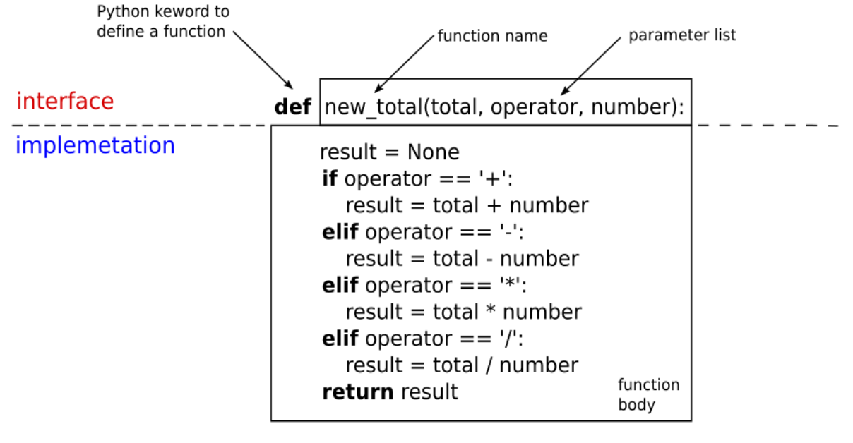
The function name, new_total, and its parameter list are visible to client code that uses the function. The function's parameters may also be referred to as its formal parameters or arguments. The function body, in the function's implementation, is hidden from client code.

Inside the function body its parameters become local variables. Such variables only exist while code in the function executes and are then gone forever. We say the scope of these variables is the function. Assigning a new value to a local variable has no effect on anything outside the function even when an external variable has the same name as the local.

The local variable result declared within the function is even more local than its parameters: there is no way the value of result can be changed externally. However, when the function is called by client code the values of the arguments to the call are passed to the function initializing its parameters to the same values as the arguments. Below old_total, operator and number are passed to new_total() and the return assigned to updated:

old_total = 101
operator = '+'
number = 7
updated = new_total(old_total, operator, number)

The arguments (old_total, operator, number) are sometimes referred to as the actual parameters of the call. The result of the function is returned to the caller where it can be assigned to a variable, used in an expression or simply discarded.

Placing the function in an expression makes assignment to an intermediate variable unnecessary

cumulative = old_total + new_total(old_total, operator, number)

But if we write

new_total(old_total, operator, number)

The function is called but its return value is not used. Doing this is pointless in this case: new_total() has no effect other than returning a value. Other functions may have useful side effects. The built in function print() for example, sends output to the screen.


The scope of variables and functions

Python requires declare before use. The scope of a variable or function is therefore from the point where it is declared or defined up to the end of the file it is declared in. When another file is imported variables and functions in that file will only be visible after the import statement. There are two import options. An entire file or files can be imported:

import math, array

but when anything from the import is referred to it must be prefixed with the file name

print(math.pi)

Alternatively, specific items from a file can be imported and optionally given an alias:

from math import sqrt, pi
from math import sqrt as root, pi as pye
print(sqrt(2))
print(root(3))
print(pi)
print(pye)

Doing this the file name prefix is not part of an item's name in the current file but all three options can be used together.

When a file is imported any executable code it contains is run to provide for initialization of variables in the import. However, execution can be made conditional by putting code, and any import directives, within an if statement:

if __name__ == '__main__':
    inc_count()
    import math
    print(math.pi)

With the __name__ condition shown code placed within the if for testing or debugging will only be run when the file itself is run not when it is imported.

Within the body of a function all items whose scope it falls within are visible. Any external function can be called and there is read only access to external variables. Optionally a function can be given additional write access to a variable by declaring it global within the body:

count = 0
def inc_count():
    global count
    count += 1 # read this as increment count by 1

Possibly useful for file initialization, maintaining a counter for debugging or performance evaluation but generally to be avoided, I think.


Function return values

A return statement in a function stops its further execution and the value from any variable or expression that follows the return is passed back to the caller. There is of course a variation to this no further execution rule. When the return is inside a try - finally block, code in the finally part will be executed come what may. This option can be left aside for the present.

There can be as many return statements in a function as required each return representing a separate exit point. Using this style new_total() can be implemented as

def new_total(total, operator, number):
    if operator == '+':
        return total + number
    if operator == '-':
        return total - number
    # etc.
    return None

When operator is not a '-' execution drops through to the next test of operator, and so on. The elif: (else if) can be replaced with a simple if: there is no need to step over tests that follow when a return takes care of a success.

The return None statement is in fact redundant. When a function does not contain a return statement or return has nothing to return, None is returned by default. You can see None being returned by a built-in function that only produces a side effect and has nothing to return by executing print(print()).

However, returning None, perhaps to show that none of the conditions in a function was True, the return needs to be explicit for clarity as to what is intended. By returning None we can write

result = new_total(old_total, operator, number)

if result != None:
... # some actions
else:
... # some other actions

Because None is logically equivalent to False in Python, we could write if result: ... but doing that is probably going to be wrong. A zero value, integer or floating-point, also has a logical equivalent of False so the else actions will be selected for all these cases. If that is the requirement then a remark in the code to explain this is essential but that will mean just as much typing as putting both conditions into if not (result == None or result == 0):.


Using single or multiple exit points

The opinion that a function should only have a single exit point is sometimes seen. This idea probably dates back to a very long time ago and supporters of old style Pascal. At that time Pascal was a language from academia that attempted to promote structured programming by enforcing a single exit at the end of a function, as opposed to C a language designed to cater for a specific range of needs in real world programming.

As far as I can see a single exit has nothing to do with structured programming. Execution in a function with multiple exit points follows the form of a tree. In an equivalent with a single exit point execution tends to the form a graph with nodes linked back to the trunk, an altogether more complex structure. Introducing variables only required to hold a return value until the end of the function introduces more clutter and room for error.

The only advantage of a single exit was simplification of resource deallocation by putting it at a single point, a non-requirement when try - finally and garbage collection is available. Go for simplicity and clarity over opinion with no logical basis and use single or multiple exit points as indicated to get these requirements, maybe?


Mutable and immutable

All the types we have looked at so far, integers, real numbers and strings, are strict values. Such values are immutable: they cannot be modified. Changing the value of the number 2 to make it 3 so all twos in a program become threes is an obvious absurdity. It should not be and is not allowed. We can change the value at a variable by assigning a new value but the value itself is inviolate.

This is not the case with all types. Some types are mutable and allow their content to be changed. When an instance of one of these types is assigned to a variable a reference to the instance is assigned. Assignment from that variable to another variable copies the reference and both variables now refer to the same instance.

Not surprisingly modifications to an instance from one variable are seen from all the variables that hold a reference to it. Similarly, when a reference to a mutable type is passed as an argument to a function, modifications to it as a local variable are reflected to all other references. Some locals are more local than others.

The built-in type list is mutable. It supplies a sequence of any type and elements can be modified by indexing into the list and assigning new values. In common with all similar Python types indexing is zero based, the first element is at index [0]. For example:

def increment_elements(numbers_list):
    index = 0
    for number in numbers_list:
numbers_list[index] = number + 1
index += 1

a_list = [1, 2, 3, 4]
increment_elements(a_list)
print(a_list)

output: [2, 3, 4, 5]

As can be seen modifications in the function increment_elements are seen from the variable a_list. Each iteration of the for loop assigns successive elements of the list to num. The loop can be made slightly neater by using the built-in function enumerate that returns both the element and its index:

def increment_elements(numbers_list):
    for index, number in enumerate(numbers_list):
a_list[index] = number + 1

The enumerate() function complies with the single return rule by returning a tuple. The tuple is unpacked transparently to the variables index and number.

A tuple is similar to a list - elements have a specific and usually a meaningful order, but a tuple is immutable once created.


Summary

Here we have looked at the usage and structure of functions and the scope of entities within a program including local and other variables. Algorithms 4 looks at functions with an indeterminate number of parameters. Lazy evaluation and closures will be considered in Algorithms 5.

[Algorithms 3: Functional integrity   (c) Martin Humby 2015]

Permalink Add your comment
Share post
ExLibris

Algorithms 2: An invariant Greeting

Visible to anyone in the world
Edited by Martin Thomas Humby, Sunday, 26 Jul 2015, 21:43

The exit behaviour problem found with the 'Greeting' program in Algorithms 1 was down to incorrect ordering of statements inside the while loop. To solve this problem start again and do a proper job this time.

Step 1: Write a general description of what we want the algorithm to do and how it might do it; call this an 'initial insight' if you so wish:

Output a general greeting statement. Read in a user's name and if the input is not an empty string output a more specific greeting that includes the name. Keep on doing these last two actions until an empty string is input.

Step 2: An algorithm is a list of precise instructions for solving a problem. All instructions must be unambiguous. By definition anything written in an entirely formal language like a programming language is unambiguous but this does not mean such a listing will match what is required or make it easy to see what went wrong when it doesn't.

Some intermediate form written more in the language of the problem than that of the implementation is often useful but the variety of styles for writing such algorithmic statements are numerous. Currently a pseudocode, formal English, style seems to be becoming more general than numbered lines with gotos so following this trend:

    Output a general greeting

loop
Request a name and read it in
if name is an empty string
break # break means exit the enclosing loop
Output a greeting that includes name
# the end of the loop

Output a goodbye message

Step 3: implement the code. Start PyCharm, the Greeting project is open or if you have closed it to start another select it from File >  Reopen Project. Select hello.py in the project tree and do Ctrl + C (copy). Select Greeting in the project tree and do Ctrl + V (paste) naming the new Python file, 'hello2.py' say. Edit code in the new file to be as follows:

print("Hello, g'day, its great to see you")
while True:
name =
input('Please input your name >')
 if
name == '':
       
break
  
print('Hello', name + '. Welcome to algorithms and data structures in Python.\n')
print('\nBye')

Run hello2.py by right click on the new file in the edit window or on the project tree. Everything works as might be expected.

Python does not have a loop or a repeat..until. To locate a loop condition anywhere than at the apparent start use while True (loop forever) with break to get a conditional exit from the loop. In print('Hello', name + '. Welcome to algorithms and data structures in Python.\n') the string concatenation operator + is used to join name to the string literal and get the full-stop in the right place; \n includes a new line character in output.


A loop invariant

There is a property of loops called the loop invariant that guarantees correct working when chosen to relate to the task the loop performs (actually it only guarantees partial correctness because it does not ensure the loop will ever terminate, but that is something else). We already know that the loop in hello2.py works as required but a check that it complies with an invariant property may be instructive particularly in view of the perhaps unusual location of the loop condition.

The invariant must hold - be true, before and after each repetition of the loop (aka. an iteration). Basically this means that it must hold before the test allowing loop entry or re-entry and hold after this test whether or not the test returns true. The invariant for a loop summing a list of numbers, for example, states that the total of those already summed and those still to be summed is constant and equal to the eventual summation: the required result towards which the loop progresses.

Python does not allow assignments or other operations in conditions so it is unlikely that a simple loop-entry test will result in an invariant failure after the test when the invariant holds before it. However, as we will see later, side effects from calling a method of an object could result in a fail so the before and after requirement is worth keeping in mind.

So, what is the loop invariant for hello2.py? A possible requirement is that the variable name should hold a string with length greater than or equal to zero. This is far too weak: all strings have a length greater than or equal to zero.

A good invariant is that name must hold a string read anew from user input on each iteration. We could say that the required result embodied in the total of the invariant and the exit condition, the result the loop must progress towards, is that the user becomes more and more bored with inputting names and eventually presses return without entering one. The Algorithms 1 Greeting did not comply with this invariant helping me to write flawed code in hello.py.

In 'hello2.py' the invariant holds before and after if name == '':. and the location of the loop test is perfectly sound. The test marks the loop entry and re-entry point where the invariant must hold, while is just the point on the loop that execution jumps back to after each iteration. Any reasonable compiler will remove the while check that True is true and jump execution back to the input statement.

When the initial assignment to name takes place the loop has not been entered despite the fact the assignment appears after the while. To locate the test with while and maintain the loop invariant, name must be initialized with a user input before the loop:

name = input('Please input your name >')
while name != '':
   
print('Hello', name + '. Welcome to algorithms and data structures in Python.\n')
  
name = input('Please input your name > ')

There is nothing wrong with this version, in fact it looks somewhat neater than the original but that is down to Python syntax rather than any problem with the original code. Whether it is easier to read, having greater clarity, is a matter of opinion and possibly depends on what one is accustomed to. If the initial insight indicates a loop-exit located other than with the while why not put it there, maybe?


In this offering we have looked at three aids to developing correct algorithms: initial insight, pseudocode and loop invariants. I hinted that initial insight should include a specification of what the algorithm must do or achieve. This requirement ensures that we write the right algorithm, one that solves the problem we want it to. Pseudocode and loop invariants help us write the algorithm right. (Adages adapted from validation and verification of software systems as in Boehm 1979).

Reference

    Boehm, B. W. (1979) 'Guidelines for Verifying and Validating Software Requirements
 and Design Specifications', TRW Redondo Beach, CA, USA [Online].
Available at http://csse.usc.edu/csse/TECHRPTS/1979/usccse79-501/usccse79-501.pdf
(Accessed 22 June 2015)
[Algorithms 2: An invariant Greeting(c) Martin Humby 2015]


Permalink 2 comments (latest comment by Martin Thomas Humby, Sunday, 28 Jun 2015, 13:00)
Share post
ExLibris

Algorithms 1: Algorithms and data structures

Visible to anyone in the world
Edited by Martin Thomas Humby, Monday, 3 Aug 2015, 11:40

According to Niklaus Wirth, 'Algorithms plus Data Structures equals Programs' (Wirth 1976). Efficient and well constructed programs are an ongoing interest of mine so doing a series of blogs on this subject will provide an archive and an aid mémoire for what I have found out so far.

The easy to learn programming language Python looks to be favourite for implementing the algorithms and will be the main language used. Python has fewer gotchas and 'must do it this ways' than any other I have come across. The fewer the language features to get in the way the more scope there will be for the algorithms, or that is what I am hoping. To keep things simple Windows will be the host operating system unless there is a good reason otherwise.

The only prior knowledge assumed will be a general idea of the basic flow of control structures found in all mainstream programming languages: if something do this, else do that, and repeating actions while a particular condition applies. Other assumed prerequisites will be some acquaintance with the mathematical entities integer, real number, set and sequence and an understanding that in computing terms a string is a sequence of characters 'abc def', not something that holds up your tracksuit trousers.


Getting started

I am not among those who believe that typing code into a text editor and running it with the interpreter from the command line makes you a better person. This means the first requirement is for an Integrated Development Environment (IDE) to manage and debug the Python code as it is developed.

Jetbrains PyCharm is an easy to use IDE providing good functionality straight out of the box, no plugins required, and is the best bet to make a start with I think. Initially CPython will be used. This Python version incorporates the latest language revisions as they are agreed. It provides multithreading but does not support multiprocessing - only one thread can run at any one time. To investigate parallel algorithms another version will be needed. This may mean using a different IDE, but for the present let's keep it simple. Best to download and save the required installers before running them just in case something goes wrong.

The IDE requires Java version 6+ so go to http://www.oracle.com/technetwork/java/javase/downloads/jdk8-downloads-2133151.html or where ever. This Java Development Kit (JDK) download includes the runtime environment (JRE) needed to run Java programs. Initially I will be using the 32 bit x86 version under Windows 7. Run this installer accepting default settings when offered.

Next go to https://www.python.org/downloads/windows/ and click on the latest stable release of Python 3 (at the top of the page).

Currently the link wil take you to https://www.python.org/downloads/release/python-343/ Select the installation for your machine (near the bottom of the page) Windows x86-64 MSI installer for a64 bit Windows. I ran Windows x86 MSI installer under 32 bit Windows 7. Generally accept defaults for installation but in the second dialogue that appears, 'Customize Python 3.4.3',Scroll down the list of options and turn on Add python.exe to path. A detailed installation guide can be found at http://www.howtogeek.com/197947/how-to-install-python-on-windows/

Having installed Java and Python we are ready to install the IDE. Download PyCharm Community Edition from https://www.jetbrains.com/pycharm/download/ and run the installer. Accept defaults but on the second screen check the box to associate the IDE with .py Python files. When installation finishes check the box to run PyCharm. Accept defaults and eventually a dialogue opens. Click Create New Project and an oversized approximation of the New Project dialogue we will be using from now on appears. 

Initial Project

The point to note is that the text in the top edit box includes the project title at the end. Change this text to your version of C:\Users\Martin\PycharmProjects\ALGORITHMS\Greeting, maybe?

Create the project and after its initial 'Indexing', taking PyCharm quite some time, you should see something like that shown below. The tab bars at the bottom and side can be hidden or shown by clicking the icon that looks a bit like a grey monitor in the bottom left corner and the tabs themselves dragged into position at the ends of the bars or between bars according to taste.

Add a file

If the project tree is not visible it can be shown by clicking the Project tab or double clicking on the project folder in the tool bar labelled Greeting. Right click on Greeting in the project tree (not the Greeting on the tool bar) to get the context menu and select New > Python File as shown. Name this file 'hello' and it opens in the editor window.


A greeting algorithm

As a starting point a simple requirement might be to develop an algorithm that will read in the names of any users who happen to be around and output a greeting that includes the user's name. If no name is input when the return ('Enter') key is pressed the program that implements the algorithm terminates.

A first stab at doing this might be the following lines of Python code:

print("Hello, g'day, its great to see you\n")

while
name != '': # while name is not equal to an empty string
  
name = input('Please input your name >')
   
print('Hello', name)
print('
Welcome to algorithms and data structures in Python.\n')

print
('\nBye')

Readers who are already acquainted with Python can skip this section, otherwise a few features are worth noting:

print() is a built in function so there is no need to write it or import it from somewhere else (in fact it is imported by default from a package 'builtins'), The print() function simply outputs whatever arguments are passed to it, as many as you like. By default the results of these arguments are separated by spaces in output and print() puts the cursor on a new line afterwards but this behaviour is easily modified. input('user prompt ') is another built-in function to read user input.

When looking at Python code posted on the internet much of this is in older versions of Python. Prior to version 3 print was an operator - print 'something'. This code will get an error under 3 but is easily fixed by inserting brackets - print('something').

The # character indicates the start of a remark or comment: explanatory text not executed when the program runs.

"Hello, g'day and great to see you!" is a string literal. Such strings can be enclosed in double quotes " ", in which case the string can include single quotes as in "g'day". Alternatively the start and end of the string can be indicated by single quotes and it can contain " characters.  '\n' included in a string represents a new-line character over and above anything print()may add to output.

In Python each line of code generally comprises a program statement. To start a new statement simply put it on a new line. Terminators such as ; are not required but a semicolon can be used to separate multiple statements on the same line if you must. Very long statements can go on multiple lines joined by a back-slash \ but this is seldom required and is not always compulsory.

Compound statements, like while are terminated with a colon :The body of the statement is defined by indentation, no curly brackets or begin ... end required. Thus indentation is critical, it is the only indication of the statements forming part of a compound block and separates those statements from any statements that follow, not part of the block. In 'hello.py' above the compound while includes the three indented lines of code.print('Bye') is not part of the while and is not indented. Python compound statements are:

    while <condition>:
for <a_variable> {,<a_variable>} in <interval | sequence | set>:

if <condition>:
elif <condition>: # else-if
else:

try:
except [<exception class>[as <variable>]{,<exception class>[as <variable>]}] :
finally:

with <an object> [as <variable>]:

def <a_function>:
class <a_class>:

In these definitions < > brackets enclose an item description and are not Python syntax. Likewise | indicates alternatives, [ ] brackets enclose an optional inclusion and { } braces enclose an option repeated as many times as may be required. Above, the last two cases are function and class definitions respectively, rather than executable compound statements as such but the indentation rules still apply.

Using the IDE the Tab key inserts an indentation at the cursor, the delete back-arrow key deletes the entire indentation and Shift + Tab removes an indentation from the line the cursor is on. If one or more lines are highlighted by dragging the cursor all the selected lines are relocated with Tab or Shift + Tab, handy when major code restructuring is required. Try highlighting the three lines of code after the while and shifting them around, for example.

Add the Python code shown above to hello.py.


Running the program

The next step is to run the Greeting program and see what happens. Any Python file, also referred to as a script, can be run as it stands. No need for a main() function or a program file. The Python interpreter simply starts at the top of the page and works down executing any executable statements it finds on the way, looping and/or branching as directed by the code. If any other files are referenced in import directives these files are accessed when the import is encountered. Imports can go anywhere in a file but the default import of 'builtins' can be thought of as being right at the top of the page.

There are many ways of running a script from the IDE. A straightforward way is to right click on a file that is open in the editor or on the file-name in the project tree and select Run 'hello' from the context menu (next to the green triangle). Do this and an error message appears

Error message

The variable name is not defined. Reading down from the top 'name' has not been encountered before the while loop entry condition is found. As far as the interpreter is concerned this variable simply does not exist. Double click on the file path underlined in blue and the IDE will put the cursor at the start of the line where the error was found. If the required file is not open in the editor it is opened.

To overcome this problem something needs to be assigned to name before the while. Anything will get an entry to the loop apart from the empty string ''.. As can be seen from the assignment to name from the input() function, the assignment operator in Python is  = . We could write

    name = 42

This assignment can be read as 'Let name equal 42' or 'Name takes the value 42'. Some people like 'Name becomes 42' but this is too mushy for my taste: name doesn't become 42, it is still the variable name before and after the assignment.

Python makes no objection to the same variable holding an integer in one place, a string in another or any other type somewhere else but whether it is sensible to use this facility is another question. A general solution for the current requirement is to use the special object None. A variable holding None is never equal to any other variable except another one holding None.

Before the while type in the line

    name = None

Run 'hello.py' again and the 'Please input your name >' prompt appears. To input names click in the Run pane to relocate the cursor, type in the name and hit return. Do not worry when the cursor appears before the prompt, typing anything puts it in the right place. The program runs successfully and exits when return is pressed without typing a name. However, its exit behaviour is not really what is required.

If it is possible to mess up something this simple perhaps there is more to this algorithms thing that might at first be thought but further discussion will have to wait for another time.


Reference
    Wirth 1976, 'Wirth, N, Algorithms + Data Structures = Programs', Prentice Hall

[Algorithms 1: Algorithms and data structures      (c) Martin Humby 2015]


Permalink
Share post
ExLibris

Easy graph algorithms

Visible to anyone in the world
Edited by Martin Thomas Humby, Tuesday, 7 Apr 2015, 23:03

A Python implementation of a generic graph structure makes various algorithms from M269 Unit 5 easy to understand.

A graph comprises nodes (aka vertices) representing entities and edges, conceptualized as lines joining the nodes and representing the relationships between them. In real world applications the graph can model a situation involving relationships between concrete entities: towns and the roads between them, connection points on a PCB or microchip, buildings requiring provision of a cabled or piped service, the sides and base of a folded metal part, super-pixels in an image used for object recognition, and so on.

A graph can be directed: its edges can be traversed in only one direction, or not: two way traversal is permitted. Edge traversal may involve a cost and edges can have a weight representing this cost. A single edge joins only two nodes and where there is no relationship between the two no edge joins them.

In this implementation nodes are represented by a base class Vertex:

class Vertex( ):
    def __init__(self, name, ID):
        self.ID = ID                # integer identifier mapped to/from name
        self.name = name            # any or multiple types relating to the application
        self.edges = StableSet()    # addition order of vertices in the set is maintained
        self.distance = 0           # basic attribute e.g distance from nearest town

Edges are represented by an Edge class:

class Edge( ):
    def __init__(self, toVertex, delta = 0):
        self.toVertex = toVertex    # the vertex at the far end of this edge
        self.weight = weight        # the weight, cost, distanced got by traversing

By default a Graph object is directed – edges run in only a single direction toVertex, but a graph can be constructed as not-directed. When edges are added to a not-directed graph the vertices they reference are added, as for directed, but edges running in the reverse direction are also put to the set of edges for each additional node.

When a vertex is added to a graph any type can be used as its 'name': the identifier apparent to users.  A name is maintained as unique as is the integer identifier it maps to.

A sensible way to construct the graph from Unit 5 Figure 5.20 is

g = Graph(directed = False)
g.addEdges('w', ('u',2), ('z',4), ('x',2))
g.addEdges('x', ('v',6), ('y',3))
g.addEdges('u', ('v',1))
g.addEdges('y', ('v',5))
g.addEdges('v', ('y',5))
g.addEdges('z', ('y',1), ('v',6))

but

g.addEdges('w', ('x',2), ('z',4))
g.addEdges('x', ('v',6), ('y',3))
etc........... then
g.addEdges('w', ('u',2))

gets much the same graph although algorithms such as depth first show different output because edges in the StableSet are in a different sequence and vertices are found in a different order:

['w', 'u', 'v', 'x', 'y', 'z'] vs. ['w', 'x', 'v', 'u', 'y', 'z']

To provide additional vertex attributes, as needed by Prim's algorithm for example, an extended class can be used:

class PrimsVertex(Vertex):
    def __init__(self, name, ID):
        Vertex.__init__(self, name, ID)
        self.currentNearest = None

A Graph will construct any class of vertex or edge passed to its constructor. Now we can define Prim's algorithm as

Add the graph vertices to a minimum-priority queue with a start node distance zero, the rest with distance infinity.
While there are vertices in the queue:

Dequeue a current-vertex and examine its edges. If any edge-weight to another node is less than the other node's distance and the other is still in the queue update its distance changing its queue position and set its currentNearest vertex to the current-vertex.

The node at the front of the queue now carries the minimum distance to get to it from any node and thus from its currentNearest so append the edge, front's currentNearest -> front-node, to a list of such edges.

Join up the edges in the edge list by matching start node to end node to get a new graph, the minimum spanning tree of the original.

 General application

This project was implemented as a quick guide to Unit 5 graph algorithms. To make it generally applicable some modification might be good. Name mapping to integers looks OK: vertices are in a lookup table getting fast access through the graph structure. Implementing not-directed using double directed edges is an easy way to do it. Whether this will get any snags for more advanced work is unknown.

Adding algorithm specific attributes by sub-classing is not generally applicable I would think. Could be better to handle these by making the algorithm function add these attributes and delete them afterwards.  The current minimum-priority queue is probably more a good laugh than a serious contender.

Single class implications

In current Python an object can be given a new attribute at any time simply by assigning a value to it, and subsequently removed using del()

    an_object.newAttribute = 0;    del(an_object.newAttribute) 

This works with new or old-style objects. Providing the multipurpose Vertex.distance field is retained so that comparison works as before the impact on the algorithms from using this strategy is generally minimal. The exception is topological-sort requiring no less than four loops through the entire graph to deal with the required incoming edges attribute.

The zip has been updated to include these investigations in TopSort2.py, Prims2.py, etc.

To deal with TopSort requirements looked at some variations to Graph and Vertex and included a fromVertex attribute for Edge and an in_edges attribute for Vertex. Initial TopSort incoming is now aVertex.in_order(). These variations are in Graphs3.zip

Permalink Add your comment
Share post
Attachments:
application/zipAVLTree.zip
ExLibris

An AVL Tree in Python

Visible to anyone in the world
Edited by Martin Thomas Humby, Wednesday, 1 Apr 2015, 14:16

Seems to me that the workings of an AVL self balancing binary search tree are easier to understand if all functionality is either in the tree or in the nodes, one or the other.

Node functionality fits well when using recursion to navigate the tree but has the disadvantage that for an empty tree the root is null. Thus we see code in the tree itself with most method bodies prefixed with

    if root != None:

This implementation uses dynamic dispatch to overcome this problem. It features three classes of 'node': EmptyTree, a RootNode and Node. The behaviour of methods such as put(), to add a new key-data pair to the tree, and remove(key) vary according to the class of node they are called against.

If put(key, data) is called against an EmptyTree at the root, it creates a new RootNode using the key-data and assigns it to the root. When the tree becomes empty because all the nodes have been deleted the RootNode assigns an EmptyTree.

The power of Python allows the AVLTree class to be implemented without writing numerous methods that call the root. A single method binds the current root and its public methods to appropriately named instance variables:

class AVLTree():
    def __init__(self):
        self.root = EmptyTree(self)
        self.setBindings()

    def setBindings(self):
        self.isEmpty = self.root.isEmpty
        self.clear = self.root.clear
        self.put = self.root.put
        self.putTuple = self.root.putTuple
        self.putKeys = self.root.putKeys
        self.putIt = self.root.putIt
        self.get = self.root.get
        self.remove = self.root.remove

    def __iter__(self):
        return self.root.__iter__()

    def __bool__(self):
        return not self.isEmpty()

Everything else is hidden and access to the root is completely transparent. A method call is anAVLTree.put(key, data) for example, where anAVLTree is an instance of the class. Binding and rebinding only takes place when the tree's state changes from empty to not-empty or vice versa, infrequent events for most applications.

The code is in the zip. If you would like to have a look extract all files to the same folder. A few points: if something: is used rather than if something != None: or if something != []: etc. I also make use of the fact that int(aBoolean) gets 1 if aBoolean is True, 0 otherwise, thus

    def put(self, key, data = None, parent = None):
    # return 1 if the height of the subtree from this node has increased, 0 otherwise
        ..........
        balance = self.balance
        if key < self.key:
            if self.leftChild:
                self.balance += self.leftChild.put(key, data, self)
        ..........etc.
        return int(self.balance != balance and self.balance != 0)

And then of course there is += equivalent to Delphi's inc(a, byB) that may be unfamiliar to those who feel traditional Pascal represents a good style  ........
 
A complete explanation of adjusting balance after a rotation can be found at (Brad Appleton 1997) but note that Brad uses right_height left_height to determine balance while, by following maths' anticlockwise tradition and Wikipedia, I have ended up with the opposite.

One interesting point was that although in-order iteration while deleting nodes in the loop does not work (some nodes are not found) by doing this the tree is not corrupted. However, because I have used single linking, the tree can be cleared by assigning an empty tree to the root and in CPython all its nodes should be deallocated without waiting for garbage collection.

Update, stress test added: put 100,000 records, check they are in the tree, remove them all.

I was quite impressed by the time it takes to check the 100,000. Almost no time at all!


Permalink Add your comment
Share post

This blog might contain posts that are only visible to logged-in users, or where only logged-in users can comment. If you have an account on the system, please log in for full access.

Total visits to this blog: 74784