Personal Blogs

Arrays and records supply primitive data structures that can be used to construct other more complex types. As they stand these basic structures form part of several algorithms and make a good place to start.

An array is a monolithic sequence of elements usually all of the same type. Ordering of elements is sequential so they can be addressed by one or more indices that identify a particular element. It makes sense to to refer to the arrangement of elements as being in a line even when the line has a number of disjunctions to produce rectangular or other shapes. Always there are first and last elements and, for inner elements, next and previous elements. These properties make arrays one of a group known as linear data structures.

The elements of a record, generally referred to as its fields or members, may or may not be of the same type and are addressed through identifiers, typically a name. The arrangement of fields in a record can be seen as forming a tree with identifiers holding an offset from its base. This is a somewhat unusual view but illustrates the fact that records are not linear as such.

Arrays

Consider an array that has been initialized so that all its elements contain an integer value of zero as shown below. The indices to elements have been included for convenience and the array has been assigned to an identifier an_array making it accessible:

In many languages creating this array would mean that all its zeros were contained in a single contiguous block of memory with all bytes set to zero. Python does provide this kind of array with its array type initialized to hold integers but I want an array capable of holding any type including records and supplying the option of multiple dimensions. Arrays with these capabilities can be got from array_types.py in the Arrays.zip attachment.

Initializing one of these arrays with integers the result is as shown below:

The array comprises a contiguous block of references all pointing to the one and only int(0) object supplied by Python. This difference is of no great importance because integers and their like are immutable. One integer zero is as good as any other or indeed the same one.

Arrays are accessed by indexing into the array. To get the 10th element of a one dimensional array, also called a vector we write:

element_10 = an_array[9]

The variable element_10 now holds a reference to the same data as the tenth element of an_array, which may or may not be mutable. With the single proviso that modifying a mutable element can have external effects, an array can be viewed as holding its elements directly or holding references to those elements. The same is true of any variable.

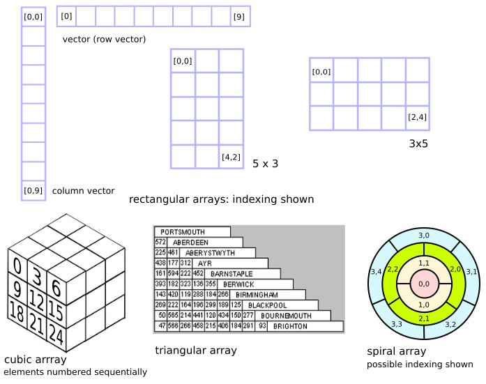
Arrays may have one, two or more dimensions and boundaries that are not rectangular. Elements can form a triangle or a spiral arrangement for example:

In all cases there must be a unique mapping between the one or more indices and the elements of the array. A spiral type could map by [layer, element-in-layer]. Gaps in the elements mapped in the underlying array may be of no concern. The fact that index zero in a vector is not used is preferable to subtracting 1 from all indices when they are used with the array. Mapping the years 2000 to 2015 to array elements simply requires subtracting 2000 from submitted indices but the series 2000, 2005, 2010, .... indicates using a bit more arithmetic.

The array type in arrays.py is called array_ to distinguish it from Python's type. To create an instance of a 3 x 3 x 3 cubic array the syntax is

array_3D = array_(3, 3, 3, numbered=True) # number each element sequentially
array_3D[0, 0, 0] = 'first'
array_3D[2, 2, 2] = 'last'
print(array_3D[0, 0, 0], array_3D[2, 2, 2], '\n\n', array_3D) 

This syntax is typical of languages that provide multi dimensional monolithic arrays, Pascal for example. It is not the norm in Python because it does not provide these types out of the box. But no worries, the syntax for accessing elements of arrays with one dimension is identical in both cases. Python lists and arrays will be discussed at a later time.

To get the software into your equivalent of C:\Users\Martin\PycharmProjects\ALGORITHMS\Arrays and records follow a similar procedure to that given for Truth Tables in Algorithms 5:

Array visualization

Perhaps you might care to experiment by instantiating some larger arrays and printing them. Maybe assign a marker string to an element and see where it occurs in the printout. A few examples are in array_types.pi. To limit the number of different instances printed at any one time PyCharm provides a useful facility for inserting or removing # from lines of code so they are executed or not: highlight all or part of each line and press Ctrl +  /.

 [0, 1, 2, 
  3, 4, 5, 
  6, 7, 8, 

  9, 10, 11,
  12, #, 14, 
  15, 16, 17, 
 
  18, 19, 20, 
  21, 22, 23, 
  24, 25, 26]

Any array from a printout arranged as shown above (but with the # put in quotes) can be assigned to an array with the same number of elements:

an_array.assign([0, 1, 2, .... # etc.

Lookup tables

Arrays provide the fastest possible access to data that can be arranged sequentially on some ordinal. Ordinals are subsets of the ordinal numbers {0, 1, 2, ...} but other values can be mapped to them. The set of characters can be mapped directly to the ordinals. Strings cannot because they do not have a fixed length. While they can be placed in alphabetical order there can be any number of strings over an interval from 'A' to 'B', say.

Values that can be mapped to ordinals must have a least term and each subsequent term must have a fixed relationship with the previous term or terms. Generally,  where  is some function. Where mappings are not unique, the case of 2000, 2005, 2010, ... for example, the consequences must be known and taken into account when a value is looked-up in the array. A lookup of 2003 could generate an error, return the value for 2000 or alternatively for 2005 or some interpolation could be applied.

The kind of data that can benefit from storage and lookup in an array are values that cannot be computed because they result from external factors and values from long and complex calculations that are used frequently. Distances between towns on a map or locations on a PCB layout, for example, can be stored in a two dimensional array so that the most economical rout covering a number of points can be found. Integers can be mapped to town names. During computations the fact that town 3 is 'Ayr' is unimportant. To provide human readable output another lookup-table index to name can be generated.

Because the distance A to B is the same as B to A, a square array gives more than 50% redundancy. For an additional overhead when looking up a distance a triangular array can be used. As for any multidimensional array a function that will map indices in the multidimensional space to an index in the underlying vector of values is needed.

In two dimensions the requirement is for the number of elements in preceding rows plus elements in the current row. Zero based indexing simplifies the calculation getting row_index * row_size + column_index for a rectangular array. In a triangular array the size of each row increases:   

def _compute_index(self, indices):  # indices is a tuple
    row = indices[0]
    column = indices[1]
    if column > row:
        row, column = column, row   # swap row with column
    row_total = (row-1)* row // 2
    return row_total + column

Referring to the distance map in the figure above PORTSMOUTH at index [0] has a row size of zero: a virtual row. Row sizes form an arithmetic series with sum number_of_terms * (first_term + last_term) / 2.  First term is zero but we want want the sum of preceding rows and because row [1] ABERDEEN maps to row zero in the underlying array subtract 1 from the row index to get number_of_terms. Because the multiplication is done first integer division // can be used to get an integer result.

Using arrays that are not rectilinear row sizes must conform to a sequence, not necessarily linear, but one that has a closed form - a formula giving the nth term, that can be summed.

Summary

Arrays provide a simple, efficient and easily applied data type accessed by indexing. The restriction they have relates to their fixed size but it is simple to write types based on an array that provide for addition and insertion of additional elements. How this is done will be revealed in Algorithms 12. Algorithms 10 looks at the records.