12.2 The gradient of a graph
We often want to know how one quantity varies with respect to another. We may be interested in the actual value of one quantity for a particular value of the other quantity (as in Section 12.1), but it is more often the rate at which one quantity varies with respect to another that is of more importance. The slope or gradient of a graph gives us a method of finding rate of change. We have already discussed the fact that Figure 12.1 shows us that the girl’s height increased rapidly in the first couple of years and then her growth slowed down. We know this because the gradient (slope) of the graph is initially steep but then becomes shallower.
In this activity, there is only space to discuss how to find the gradient of a simple straight-line graph, such as the ones shown in Figure 12.4. A straight-line graph is one in which quantity plotted on the vertical axis varies at a steady rate with respect to the quantity plotted on the horizontal axis. In other words, the gradient of the line is constant.
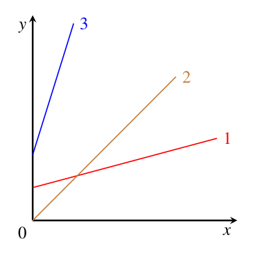
Which of the lines in Figure 12.4 has the largest gradient and which has the smallest gradient?
Line 3 has the largest gradient – this is the steepest slope. Line 1 has the smallest gradient – it has the smallest change in the vertical direction for any particular change in the horizontal direction.
The gradient of a straight line is defined as:
This is sometimes stated as:
To work out the gradient of a straight line on a graph, we simply need to take any two points on the line (to increase the precision of the calculation, the points should be quite well separated) and find the change in vertical value (the rise) corresponding to a particular change in horizontal value (the run). As an example, let’s find the gradient of the graph shown in Figure 12.5.
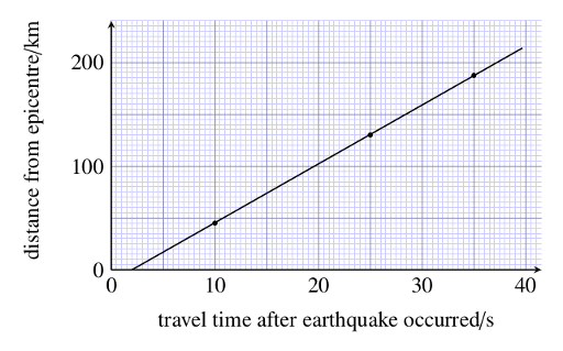
Figure 12.6 shows that as the horizontal value increases from 4 s to 32 s, the vertical value increases from 10 km to 170 km. Thus the run is (32 – 4) s = 28 s and the rise is (170 – 10) km = 160 km and the gradient is given by:
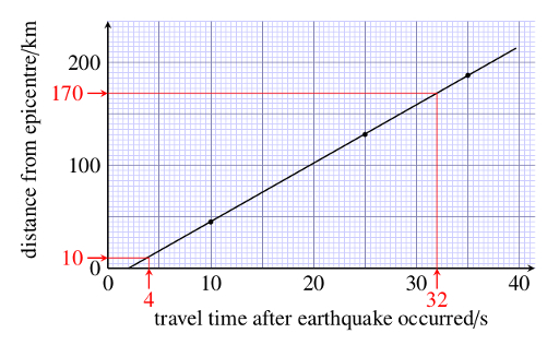
The gradient of a graph can have units, just like any other calculated quantity. In the example here, we have divided kilometres by seconds so the unit of the gradient is km s-1, which is a unit of speed. The gradient gives a measure of the speed at which the earthquake waves travel through the Earth from the epicentre to the detectors.
Note also that the rules for significant figures in calculations, introduced in Section 9.1, apply here too. In the example above, the run is given to two significant figures, so the answer is correctly given to two significant figures too.
Question 12.3
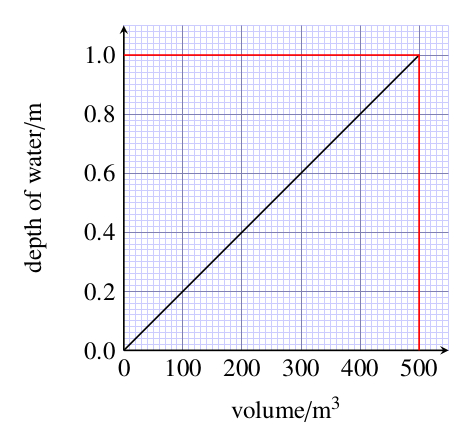
A large ornamental pool with straight sides and a flat bottom is filled with water. A meter registers the volume of water pumped into the pool. As the pool fills, the depth of water is measured. Figure 12.7 shows a graph in which the depth of water is plotted against the volume of water added. Calculate the gradient of this graph.
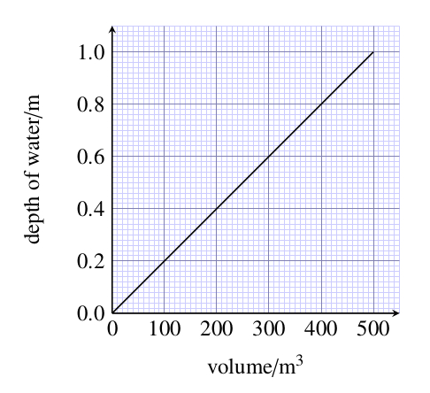 Figure 12.7 Graph for use with Question 12.3.
You may use any reasonably well separated pair of points on the graph to calculate the gradient, and should obtain approximately the same answer whichever points you choose. Taking the points corresponding to a volume of 0 m3 and a volume of 500 m3 gives: